Supervised ML/AI Breast Cancer Diagnostics

Problem

Breast cancer (BC) is the uncontrollable growth of malignant cells in the breasts [1]. BC is the most common cancer with the highest mortality rate. The exact cause of breast cancer is unknown, but some women have a higher risk than others. This includes women with a personal or family history of breast cancer and women with certain gene mutations. Since cancer cells can metastasize, or spread to other parts of the body, it’s important to recognize the symptoms of BC early on. The sooner you receive a BC Diagnosis (BCD) and start treatment, the better your outlook [2].

Conventional BCD involves imaging tests to look for BC spread. Imaging tests use x-rays, magnetic fields, sound waves, or radioactive substances to create pictures of the inside of your body. Imaging tests might be done for a number of reasons including [2]:

To look at suspicious areas that might be cancer
To learn how far cancer might have spread
To help determine if treatment is working
To look for possible signs of cancer coming back after treatment.

Despite all of these tests, providing accurate and accessible diagnoses remains a fundamental challenge for BCD. In the US alone an estimated 5% of outpatients receive the wrong diagnosis every year; these errors are particularly common when diagnosing patients with serious medical conditions, with an estimated 20% of these patients being misdiagnosed at the level of primary care and one in three of these misdiagnoses resulting in serious patient harm [3].

Solution

In fact, a large amount of data is currently available to clinicians, ranging from details of clinical symptoms to various types of biochemical assays and outputs of imaging devices such as chest x-ray, CT/MRI/PET/bone scans, ultrasound, etc. The study of relevant factors and different types of large datasets jointly offers the attractive opportunity to diagnose BC more effectively, where there are multiple possible causes of patient symptoms.

Recently, ML techniques have been successfully applied to BCD by providing an unprecedented opportunity to derive clinical insights from large-scale analysis of patient data [3, 4]. Clinical decisions have traditionally been guided by medical guidelines and accumulated experience. In contrast, ML methods add rigor to this process; algorithms can generate individualized predictions by synthesizing data across broad patient bases. Some benefits of leveraging ML in BCD are as follows [4]:

· Find risk factor (which features are most sensitive to BC)

· Increase BCD efficiency(early and accurate BCD)

· Reduce unnecessary hospital visits (only if needed).

The projections for this technology's growth in the next five years are promising, as well — in fact, researchers project a 45% growth rate for medical AI [5].

Figure 1 illustrates the most basic application of ML/AI in BCD as the binary classification problem. Classification usually refers to any kind of problem where a specific type of class label is the result to be predicted from the given input field of data. This is a task which assigns a label value (“benign” or “malignant”) to a specific class and then can identify a particular type to be of one kind or another. Generally, one is considered as the normal state and the other is considered to be the abnormal state. In BCD, ” No cancer detected” is a normal state and ” Cancer detected” represents the abnormal state. For any model, you will require a training dataset with many examples of inputs and outputs from which the model will train itself. The training data must include all the possible scenarios of the problem and must have sufficient data for each label for the model to be trained correctly. Class labels are often returned as string values and hence needs to be encoded into an integer like either representing 0 for “benign” or 1 for “malignant”. For each training example, one can also create a model which predicts the Bernoulli probability for the output. In short, it returns a discrete value [0-1] that covers all cases and will give the output as either the outcome will have a value of 1 or 0.

Figure 1 Supervised ML for BCD: classification of tumors using training data with “right answers” for each example in the data y={0,1}. Given a patient with a tumor, we have to predict whether the tumor is malignant (Yes or y=1) or benign (No or y=0). This is the binary classification problem with the discrete-valued output representing the negative class A (y=0) and the positive class C (y=1). Area B is the threshold area with 50% chance of predicting either class.

Figure 2 Supervised ML for BCD: binary classification of tumors using the most popular Support Vector Machine (SVM) algorithm. The main (One vs One) task is to define a binary model for every pair of classes. The SVM decision boundary (dashed line) has the characteristics to ignore the outlier (Bias Area) and finds the best hyperplane that maximizes the margin. That is why SVM is robust to outliers.

Figure 3 Error analysis of binary classification ML/AI using 2x2 confusion matrix with 4 values.

SVM Algorithm

Figure 2 explains the most popular Support Vector Machine (SVM) algorithm [6-14] applied to the binary BCD classification problem in Figure 1. The objective of SVM algorithm is to find a hyperplane in an N-dimensional space that distinctly classifies the data points [14]. The dimension N of the hyperplane depends upon the number of features. If the number of input features is two (N=2), then the hyperplane is just a line. If the number of input features is three (N=3), then the hyperplane becomes a 2-D plane. It becomes difficult to imagine when the number of features exceeds three. In Figure 2, we begin by adding extra features to our data such as age vs tumor size (N=2). Next, we fit the straight line (SVM decision boundary) to separate malignant tumors from benign ones. From Figure 2 it is clear that there are multiple lines (our hyperplane here is a line because we are considering only two input features such as age and tumor size) that segregates our data points or does a classification between blue circles and orange squares.

So how do we choose the best line or in general the best hyperplane that segregates our data points? The Bias Area in Figure 2 contains outliers of both binary classes. The SVM algorithm is robust to outliers in that it ignores these outliers and finds the best hyperplane or decision boundary (dashed line in Figure 2) that maximizes the margin. Specifically, SVM tries to minimize the cost function 1/margin + penalty (aka hinge loss) representing the bias area in Figure 2.

In Figure 2, we have only 2 features – the age and the size of the tumor. How about a large number of features (clump thickness, uniformity of cell size/shape, fractal dimension, etc.)? Fortunately, SVM is effective in high dimensional cases when N>>1. It is memory efficient as it uses a subset of training points in the decision function called support vectors. In addition, different kernel functions can be specified for the decision functions and it is possible to specify custom kernels [14].

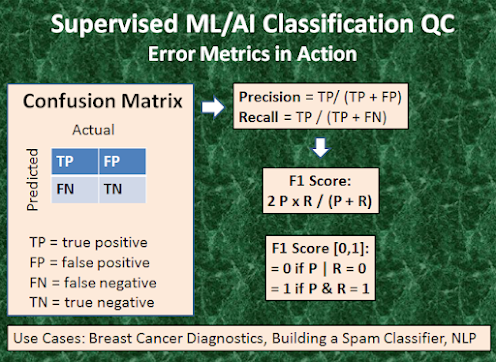
Error Analysis

A confusion matrix is an M x M matrix used for evaluating the performance of a classification model, where M is the number of target classes. For our binary classification problem, we have a 2 x 2 matrix as shown in Figure 3 with 4 values: TP, FP, FN, and TN. Let’s decipher the matrix:

· The target variable has two values, Positive or Negative;

· The columns represent the actual values of the target variable;

· The rows represent the predicted values of the target variable.

True Positive (TP)

· The predicted value matches the actual value;

· The actual value was positive and the model predicted a positive value;

True Negative (TN)

· The predicted value matches the actual value;

· The actual value was negative and the model predicted a negative value;

False Positive (FP) aka Type 1 Error

· The predicted value was falsely predicted;

· The actual value was negative but the model predicted a positive value;

False Negative (FN) aka Type 2 Error

· The predicted value was falsely predicted;

· The actual value was positive but the model predicted a negative value.

The overall performance of the ML algorithm can be assessed by means of the following fundamental QC metrics (Figure 3):

Precision (P) = TP/ (TP+FP),

Recall (R ) = TP/ (TP+FN),

Accuracy = (TP+TN)/(TP+FP+TN+FN),

F1 Score = 2*P*R/(P+R).

Precision would determine whether our model is reliable or not: of all patients where we predicted y=1, what fraction actually has BC? Recall tells us how many of the actual positive cases we were able to predict correctly with our model: of all patients that actually have BC, what fraction did we correctly detect as having BC? Accuracy 99% correct BCD means that you got 1% error on test BC set. Finally, the F1 Score [0,1] is useful when we combine precision/recall numbers while benchmarking different classification algorithms, for example. Here, the objective is to resolve the precision-recall trade-off by finding an optimal threshold TH: predict y=1 if cost function > TH. The optimal TH finds a balance between the following two goals: suppose we want to predict y=1 BC only if very confident (high P and low R); suppose we want to avoid missing too many cases of BC or avoid FN (high R and low P). P is a useful metric in cases where FP is a higher concern than FN. is important in music or video recommendation systems, e-commerce websites, etc. Wrong results could lead to customer churn and be harmful to the business. R is a useful metric in cases where FN trumps FP. Recall is important in medical cases (especially in BCD) where it doesn’t matter whether we raise a false alarm but the actual positive cases should not go undetected! In disease screening cases, R would be a better metric because we don’t want to accidentally discharge an infected person and let them mix with the healthy population thereby spreading the contagious virus. Now it is clear why Accuracy alone can be a bad metric for our training model. But there will be cases where there is no clear distinction between whether Precision is more important or Recall. What should we do in those cases? We combine them! In practice, when we try to increase the precision of our model, the recall goes down, and vice-versa. The F1-score captures both the trends in a single value [0,1] which is the harmonic mean of P and R values. It is maximum when P=R.

Bottom Line: In practice, we use F1-score in combination with other evaluation metrics mentioned above which gives us a complete picture of the result.

Figure 4 ML/AI ETL pipeline [6-14] that implements the BCD binary classification algorithm in Python. The input data set is split into the training data, test data and validation data as 70, 20 and 10% subsets, respectively.

Python Use Case

In this ML/AI BCD Python open-source project [16-24] we are going to analyze and classify BC using the public-domain BC dataset [15]. The dataset used in this story is publicly available and was created by Dr. William H. Wolberg, physician at the University Of Wisconsin Hospital at Madison, Wisconsin, USA. To create the dataset Dr. Wolberg used fluid samples, taken from patients with solid breast masses and an easy-to-use graphical computer program called Xcyt, which is capable of perform the analysis of cytological features based on a digital scan. The program uses a curve-fitting algorithm, to compute ten features from each one of the cells in the sample, than it calculates the mean value, extreme value and standard error of each feature for the image, returning a 30 real-valued vector computed for each cell nucleus:

1. radius (mean of distances from center to points on the perimeter)

2. texture (standard deviation of gray-scale values)

3. perimeter

4. area

5. smoothness (local variation in radius lengths)

6. compactness (perimeter² / area — 1.0)

7. concavity (severity of concave portions of the contour)

8. concave points (number of concave portions of the contour)

9. symmetry

10. fractal dimension (“coastline approximation” — 1)

The mean, standard error and “worst” or largest (mean of the three largest values) of these features were computed for each image, resulting in 30 features. For instance, field 3 is Mean Radius, field 13 is Radius SE, field 23 is Worst Radius.

Our objective is to create a model which will correctly classify whether the BC is of malignant or benign type. So with the help of the supervised ML ETL pipeline in Figure 4 if we can classify the patient having which type of BC, then it will be easy for doctors to provide timely treatment to patients and improve the chance of survival. The main steps of this project are outlined in Figure 4: input data preparation, editing and splitting, Exploratory Data Analysis (EDA), model training, testing, tuning, deployment, validation and inference. There are no missing or null data points of the data set.

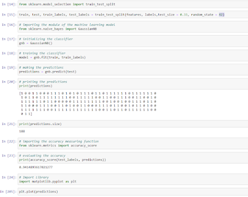
The simplest Python ETL pipeline is based on the scikit-learn library [6] available in the latest release of Anaconda IDE [7]. The corresponding Jupyter notebook Python3 sequence implements the binary classification ML algorithm as follows:

Lines 1-2 import sklearn and load_breast_cancer dataset;

Lines 3-4 store the data in a variable while creating features set and labels;

Lines 8, 9 the features type is the Numpy array;

Line 11 features size is 17070 = 569 rows x 30 columns

Line 12 feature names = 30

Line 13 view 30 features

Lines 14-15 split the data into training and test datasets (67 and 33%, respectively) by importing the function train_test_split from sklearn library;

Lines 17-18 let’s select the simplest Naive Bayes algorithm that usually performs well in binary classification tasks; firstly, import the GaussianNB module and initialize it using the GaussianNB() function; then train the model by fitting it to the data in the dataset using the fit() method;

Lines 19-21 view the predictions as 0 and 1 values;

Lines 22-23 check the accuracy;

Lines 24, 205 plot the predictions;

Lines 31-33 additional data QC views

Observed mean radius (horizontal) vs mean concavity.

Predicted mean radius (horizontal) vs mean concavity.

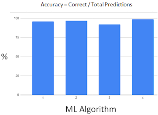
We have tried several types of classification ML algorithms (ALG):

1 Logistic Regression 95.8%

2 SVM 97.2%

3 Naive Bayes 91.6% (worst)

4 Random Forest 98.6% (best)

ALG 1 & 2 yield similar accuracy,

All ALG yield acceptable >90% accuracy.

We can make the confusion matrix

from sklearn.metrics import confusion_matrix

cm = confusion_matrix(test,predict)

sns.heatmap(cm,annot=True)

We can view it as the 2x2 table

88(87)	1(3)
2(3)	52(50)

Then we can compute the key metrics:

P=0.98 (0.96)

R=0.88 (0.96)

Hence,

F1 = 0.92 (0.96) = 0.94 +/- 0.02.

We can see that our model is working very efficiently and accurately in classifying whether the BC is of malignant type or benign type. In addition to scikit-learn, we have visualized the data using pandas and matplotlib libraries.

Technology

AWS now provides a robust, cloud-based service — Amazon SageMaker — so that developers of all skill levels can use ML technology. SageMaker API enables developers to create, train, and deploy ML models into a production-ready hosted environment.

The GCP AutoML Tables is another available supervised ML service. It requires example data to train your model by implementing the standard ML ETL pipeline in Figure 4:

1. Gather your data: Determine the data you need for training and testing your model based on the outcome you want to achieve

2. Prepare your data: Make sure your data is properly formatted before and after data import

3. Train: Set parameters and build your model

4. Evaluate: Review model metrics

5. Test: Try your model on test data

6. Deploy and predict: Make your model available to use.

Here, models can have both numerical and categorical features.

Finally, MS Azure ML Studio breaks down ML into five algorithm groups: