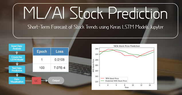
Supervised ML/AI Stock Prediction using Keras LSTM Models

 

(the image was created using Visme [1]).

Introduction

Stock markets are analyzed either technically or fundamentally [2]. Fundamental analysis studies supply and demand relationships that define the stock price at any given time. Technical analysis uses specialized methods of predicting prices by analyzing past price patterns and levels. There are many techniques used to examine stock price lines and patterns [2]:

• bar or high/low/close charts
• moving averages
• trend lines
• channels
• cycles
• resistance and support planes
• corrections
• double tops and bottoms
• head and shoulders formation
• trading volume
• open interest. 

Theere are numerous limitations of these techniques:

moving averages

• responds to general trends only
• is not highly precise
• short-term moving averages can give false indications, especially in times of volatile prices

Trend lines

• work best with sustained trends
• positioning of trend lines is subjective and takes practice
• trends must be established before they become recognizable

Channels

• work best with sustained trends, the longer the better
• positioning of the support and resistance lines is subjective and requires practice.

Cycles

• require a period of time to establish the cycle
• imprecise as time spans can vary between oscillations
• no indication as to how long the cycles will last.

Resistance or support planes

• often difficult to keep track of (not shown on charts or are off-the-scale).

Corrections

• most applicable to short term projections.

Double tops and bottoms

• usually require major resistance plane

Head and shoulders formations:

• by the time the formation is identified the trend has changed and prices moved significantly.

As fintech begins to embrace AI, supervised ML is increasingly utilized to help overcome above limitations of traditional semi-empirical time-series methods [3-5]. Although there is an abundance of historical stock data for ML to train on, a high noise to signal ratio and the multitude of market conditions cause poor predictions of stock prices. 

In this blog, let us consider a convenient solution to overcome these problems in the form of Long Short Term Memory (LSTM). LSTMs provide us with a large range of parameters such as learning rates, and input and output biases. Hence, no need for fine adjustments. The complexity to update each weight is reduced to O(1) with LSTMs, similar to that of Back Propagation Through Time (BPTT), which is an advantage. 

In LSTM NN, the past inputs to the model leave a footprint. Hence, LSTM is great tool for anything that has a sequence. 

Read more about LSTM.

The prerequisites for biotechnological production of antibiotics is

The prerequisites for this project is the Anaconda IDE with the Jupyter Python-3 notebook and the following pre-installed libraries:

import numpy as np

import matplotlib.pyplot as plt

import pandas as pd

from sklearn.preprocessing import MinMaxScaler

from keras.models import Sequential

from keras.layers import LSTM

from keras.layers import Dropout

from keras.layers import Dense

Step 1: Input Data

We can load the input data directly from the GitHub repository [5]:

url = 'https://raw.githubusercontent.com/mwitiderrick/stockprice/master/NSE-TATAGLOBAL.csv'

dataset_train = pd.read_csv(url)

training_set = dataset_train.iloc[:, 1:2].values

Let's take a look at the input data:

1. Dimensions of the dataset.
2. Peek at the data itself.
3. Statistical summary of all attributes.
4. Breakdown of the data by the class variable.

# dataframe.shape

shape = dataset_train.shape

print(shape)

(2035, 8)

# dataframe.size
size = dataset_train.size

print(size)

16280

# iterating the columns
for col in dataset_train.columns:
    print(col)
Date
Open
High
Low
Last
Close
Total Trade Quantity
Turnover (Lacs)


print(dataset_train[['Date', 'Total Trade Quantity']])

           Date  Total Trade Quantity
0     2018-09-28               3069914
1     2018-09-27               5082859
2     2018-09-26               2240909
3     2018-09-25               2349368
4     2018-09-24               3423509
...          ...                   ...
2030  2010-07-27                586100
2031  2010-07-26                658440
2032  2010-07-23                281312
2033  2010-07-22                293312
2034  2010-07-21                658666

[2035 rows x 2 columns]

Step 2: Training Model

Let's implement the following steps [3,4]:

1. Normalize the Data;

2. Incorporate Timesteps Into the Data;

3. Create the LSTM Model.

from sklearn.preprocessing import MinMaxScaler

sc = MinMaxScaler(feature_range=(0,1))

training_set_scaled = sc.fit_transform(training_set)

X_train = []

y_train = []

for i in range(60, 2035):

    X_train.append(training_set_scaled[i-60:i, 0])

    y_train.append(training_set_scaled[i, 0])

X_train, y_train = np.array(X_train), np.array(y_train)

X_train = np.reshape(X_train, (X_train.shape[0], X_train.shape[1], 1))

model = Sequential()

model.add(LSTM(units=50,return_sequences=True,input_shape=(X_train.shape[1], 1)))

model.add(Dropout(0.2))

model.add(LSTM(units=50,return_sequences=True))

model.add(Dropout(0.2))

model.add(LSTM(units=50,return_sequences=True))

model.add(Dropout(0.2))

model.add(LSTM(units=50))

model.add(Dropout(0.2))

model.add(Dense(units=1))

model.compile(optimizer='adam',loss='mean_squared_error')

model.fit(X_train,y_train,epochs=100,batch_size=32)

The above sequence implies that we apply the Adam optimizer and drop only 20% of NN layers while defining the batch size of 32. As the above plot shows, the LSTM convergence MSE Loss vs Epoch<100 is very fast. 

Step 3: Test Data

Let's apply our LSTM predictions to the real-world test dataset [5]

url = 'https://raw.githubusercontent.com/mwitiderrick/stockprice/master/tatatest.csv'

dataset_test = pd.read_csv(url)

real_stock_price = dataset_test.iloc[:, 1:2].values

The complete test sequence is listed below.

dataset_total = pd.concat((dataset_train['Open'], dataset_test['Open']), axis = 0)

inputs = dataset_total[len(dataset_total) - len(dataset_test) - 60:].values

inputs = inputs.reshape(-1,1)

inputs = sc.transform(inputs)

X_test = []

for i in range(60, 76):

    X_test.append(inputs[i-60:i, 0])

X_test = np.array(X_test)

X_test = np.reshape(X_test, (X_test.shape[0], X_test.shape[1], 1))

predicted_stock_price = model.predict(X_test)

predicted_stock_price = sc.inverse_transform(predicted_stock_price)

Results

We can evaluate the predictions by comparing predicted and actual value in the test dataset:

We can see that our model follows overall Buy/Sell Down/Up trends with some negligible fluctuations. The key takeaway is that completing a small end-to-end Jupyter project from loading the data to making predictions is the simplest way to implement AI-assisted stock predictions.

Continue reading [6]

and follow more Python ML/AI examples.

References

[1] https://www.visme.co/?ref=al24

[2] https://www.alberta.ca/how-to-use-charting-to-analyse-commodity-markets.aspx

[3] https://towardsdatascience.com/predicting-stock-prices-using-a-keras-lstm-model-4225457f0233

[4] https://becominghuman.ai/artificial-intelligence-and-its-application-in-finance-9f1e0588e777

[5] Derrick Mwiti's Bootcamp on Github

[6] https://newdigitals.org/