Real Estate Supervised ML/AI Linear Regression Revisited - USA House Price Prediction

ETL Workflow
Linear regression is an algorithm of supervised Machine Learning (ML) in which the predicted output is continuous with having a constant slope [1]. Consider a company of real estate with datasets containing the property prices of a specific region. The price of a property is based on essential factors like bedrooms, areas, and parking. Majorly, a real estate company requires [1]:
- Define the set of variables (model features like areas, number of rooms and bathroom, etc.) that affects the price of a house;
- Creating a linear model quantitatively related to the house price with model variables;
- Examine the accuracy of an output model, i.e. how well the model variables can predict the prices of a house for training, test and validation data.
So real estate experts assume that the trained, tested and deployed ML model would be capable of learning and predicting how far people would go in the bidding in order to buy a house, based on selected features. That’s the ML housing price prediction algorithm in a nutshell.
Step 1: Exploratory Data Analysis (EDA)
The public domain dataset USA_Housing.csv [2] contains 7 columns and 10000 rows with CSV extension. The data contains the following columns:
- 'Avg. Area Income' - Scaled Average Income of the householder of the city where house is located,
- 'Avg. Area House Age' - Scaled Average age of houses in the same city.
- 'Avg. Area Number of Rooms' - Scaled Average number of rooms for houses in same city.
- 'Avg. Area Number of Bedrooms' - Scaled Average number of bedrooms for houses in the same city.
- 'Area Population' - The scaled total population of the city.
- 'Price' - Scaled price that the hose sold at.
- 'Address' - Unscaled address of that house.
All attributes are numeric except for the "Address" field. Its type is an object, so it can contain any type of Python object. A quick way to get a feel for what kind of data you’re dealing with is to plot a histogram and a box/whisker plot for each numerical attribute, as shown below.


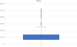
Figure 1: Histograms and box/whisker plots of raw input data [2].

The actual steps of EDA and linear regression [3] are as follows:


The sensitivity coefficient means the following:
1. Holding all the other features fixed, a 1 unit increase in Avg. Area Income is associated with an increase of $21.66.
2. Holding all the other features fixed, a 1 unit increase in Avg. Area House Age is associated with an increase of
$164990.05
3. Holding all the other features fixed, a 1 unit increase in Avg. Area Number of Rooms is associated with an increase of
$120784.23
4. Holding all the other features fixed, a 1 unit increase in Avg. Area Number of Bedrooms is associated with an increase
of $1542.52
5. Holding all the other features fixed, a 1 unit increase in Area Population of Bedrooms is associated with an increase
of $15.15
Thus, we can neglect features 1, 4 and 5 as compared to features 2 and 3.

In the above scatter X-plot, we see test versus predictions are of a line form, which means our model has done good predictions.

In the above histogram plot we see data is in bell shape(Normally Distributed), which means our model has done good predictions.


Comments
Post a Comment