Heart Failure Prediction using Supervised ML/AI Technique

Introduction
This project is aimed to support ESC guidelines [1] that help health professionals manage people with heart failure (HF) according to the best available evidence. The objective is not only to develop an accurate survival prediction model but also to discover essential factors for the survival prediction of HF patients. The complex nature of HF produces a significant amount of information that is too difficult for clinicians to process as it requires simultaneous consideration of multiple factors and their interactions [2,3]. ML/AI techniques can be utilized in this scenario to develop a reliable decision support system to assist clinicians in properly interpreting the patients’ records to make informed decisions [2-5].
Workflow
Let us install Anaconda IDE, upgrade pip and create a virtual environment Jupyter. The Python-3 ML/AI workflow consists of the following steps:
Step 1: Install/import key libraries
import numpy as np # linear algebra
import pandas as pd # data processing, CSV file I/O (e.g. pd.read_csv)
from sklearn.metrics import cohen_kappa_score
from sklearn.metrics import precision_score
from sklearn.metrics import recall_score
from sklearn.metrics import f1_score
import matplotlib.pyplot as plt
import warnings
import seaborn as sns
from colorama import Fore, Back, Style
!pip install mlxtend
!pip install plotly
from sklearn.model_selection import train_test_split
from sklearn.metrics import confusion_matrix, accuracy_score
from mlxtend.plotting import plot_confusion_matrix
from plotly.offline import plot, iplot, init_notebook_mode
import plotly.graph_objs as go
from plotly.subplots import make_subplots
import plotly.express as px
from statsmodels.formula.api import ols
import plotly.graph_objs as gobj
init_notebook_mode(connected=True)
warnings.filterwarnings("ignore")
import plotly.figure_factory as ff
%matplotlib inline
!pip install lightgbm
!pip install catboost
import xgboost
import lightgbm
from sklearn.svm import SVC
from sklearn.ensemble import GradientBoostingClassifier
from sklearn.ensemble import RandomForestClassifier
from sklearn.tree import DecisionTreeClassifier
from sklearn.neighbors import KNeighborsClassifier
from sklearn.linear_model import LogisticRegression
from catboost import CatBoostClassifier
Step 2: Download and QC input HF dataset
We work with the Kaggle Heart Failure Clinical Records Dataset [4]
Step 3: Exploratory Data Analysis (EDA)
Step 4: Feature Selection via Correlations
Step 5: Train-Test Data Split and Modeling/Prediction
Step 6: Performance Evaluation and Accuracy QC
Step 7: Confusion Matrix and Key Metrics QC
Step 8: Output Classification Report

Input Data
There are some factors that affects Death Event. This dataset contains person's information like age ,sex , blood pressure, smoke, diabetes,ejection fraction, creatinine phosphokinase, serum_creatinine, serum_sodium, time and we have to predict their DEATH EVENT:
- Sex - Gender of patient Male = 1, Female =0
- Age - Age of patient
- Diabetes - 0 = No, 1 = Yes
- Anaemia - 0 = No, 1 = Yes
- High_blood_pressure - 0 = No, 1 = Yes
- Smoking - 0 = No, 1 = Yes
- DEATH_EVENT - 0 = No, 1 = Yes

<class 'pandas.core.frame.DataFrame'>
RangeIndex: 299 entries, 0 to 298
Data columns (total 13 columns):
 #   Column                    Non-Null Count  Dtype
---  ------                    --------------  -----
 0   age                       299 non-null    float64
 1   anaemia                   299 non-null    int64
 2   creatinine_phosphokinase  299 non-null    int64
 3   diabetes                  299 non-null    int64
 4   ejection_fraction         299 non-null    int64
 5   high_blood_pressure       299 non-null    int64
 6   platelets                 299 non-null    float64
 7   serum_creatinine          299 non-null    float64
 8   serum_sodium              299 non-null    int64
 9   sex                       299 non-null    int64
 10  smoking                   299 non-null    int64
 11  time                      299 non-null    int64
 12  DEATH_EVENT               299 non-null    int64


As we can see from the output above, there are a total of 13 features and 1 target variable. Also, there are no missing values so we don’t need to take care of any null values.
The method revealed that the range of each variable is different. The maximum value of
age is 77 but for chol it is 564. Thus, feature scaling must be performed on the dataset [6].Exploratory Data Analysis
Let’s take a look at the plots below. It shows how each feature and label is distributed along different ranges, which further confirms the need for scaling. Next, wherever you see discrete bars, it basically means that each of these is actually a categorical variable. We will need to handle these categorical variables before applying ML. Our target labels have two classes, 0 for no HF and 1 for HF.
Is Age and Sex an indicator for Death Event?
- Age wise 40 to 80 the spread is High
- less than 40 age and higher than 80 age people are very low


Age Report
- Survival spread is high in age's flow of 40 to 70
- The Survival is high for both male between 50 to 60 and female's age between 60 to 70 respectively
- The Survival is high for not smoking person 55 to 65, while for smoking person it is between 50 to 60
- Death event for smoking person is high than not smoking person
- From above pie charts we can conclude that in our dataset diabetes from 203 of Non Smoking person 137 are survived and 66 are not survived and
- From 96 Smoking person 66 are survived, while 30 are not survived.
HBP
- From above pie charts we can conclude that in our dataset diabetes from 194 of Non High BP person 137 are survived and 57 are not survived and
- From 105 High BP person 66 are survived, while 39 are not survived.
Feature Engineering
Let’s see the correlation matrix of features and try to analyse it.

Accuracy Analysis
K Neighbors Classifier
This classifier looks for the classes of K nearest neighbors of a given data point and based on the majority class, it assigns a class to this data point. However, the number of neighbors can be varied. I varied them from 1 to 20 neighbors and calculated the test score in each case [6]:
# K Neighbors Classifier
kn_clf = KNeighborsClassifier(n_neighbors=6)
Support Vector Classifier
This classifier aims at forming a hyperplane that can separate the classes as much as possible by adjusting the distance between the data points and the hyperplane. There are several
kernels based on which the hyperplane is decided. I tried four kernels namely, linear, poly, rbf, and sigmoid. The linear kernel performed the best for this dataset [6]. Decision Tree Classifier
This classifier creates a decision tree based on which, it assigns the class values to each data point. Here, we can vary the maximum number of features to be considered while creating the model. I range features from 1 to 30 (the total features in the dataset after dummy columns were added).
Random Forest Classifier
This classifier takes the concept of decision trees to the next level. It creates a forest of trees where each tree is formed by a random selection of features from the total features. Here, we can vary the number of trees that will be used to predict the class. I calculate test scores over 10, 100, 200, 500 and 1000 trees. The maximum score was achieved for both 100 and 500 trees.
Cat Boost (CB)
The boosting algorithm present in the CB classifier minimizes over-fitting issues.

As one can see below, classification accuracy of up to 93% was achieved in the prediction of HF risk using the Gradient Boosting or XGBRF Classifier with this dataset.Accuracy of Logistic Regression is : 90.00%Accuracy of SVC is : 90.00%Accuracy of K Neighbors Classifier is : 91.67%Accuracy of Decision Tree Classifier is : 90.00%Accuracy of Random Forest Classifier is : 90.00%Accuracy of Gradient Boosting is : 93.33%Accuracy of XGBRFClassifier is : 93.33%Accuracy of LGBMClassifier is : 86.67%Accuracy of CatBoostClassifier is : 91.67%
Confusion Matrix
Confusion Matrix is the most effective tool to analyse HF prediction in this field of study.


Sensitivity/recall indicates the proportions of cardiac patients diagnosed by the model as with HF. Precision provides information about the proportion of those classified by the model as with HF,
had HF. F1 Score is defined as the harmonic mean of sensitivity/recall and precision assigning a single
number. Specificity indicates the proportions of patients not having HF been forecasted by the model to
the category of non-cardiac disease.
log_reg_pred
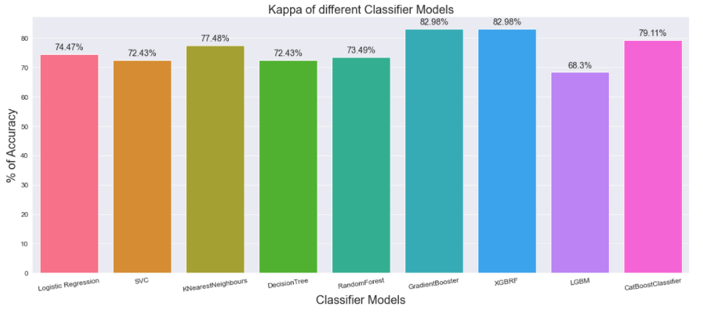
Precision: 0.866667
Recall: 0.764706
F1 score: 0.812500
Cohens kappa: 0.744681
sv_clf_predPrecision: 1.000000 Recall: 0.647059 F1 score: 0.785714 Cohens kappa: 0.724349kn_predPrecision: 1.000000 Recall: 0.705882 F1 score: 0.827586 Cohens kappa: 0.774775dt_predPrecision: 1.000000 Recall: 0.647059 F1 score: 0.785714 Cohens kappa: 0.724349r_predPrecision: 0.923077 Recall: 0.705882 F1 score: 0.800000 Cohens kappa: 0.734904gradientboost_predPrecision: 0.933333 Recall: 0.823529 F1 score: 0.875000 Cohens kappa: 0.829787xgb_predPrecision: 0.933333 Recall: 0.823529 F1 score: 0.875000 Cohens kappa: 0.829787lgb_predPrecision: 0.736842 Recall: 0.823529 F1 score: 0.777778 Cohens kappa: 0.682959cat_predPrecision: 0.875000 Recall: 0.823529 F1 score: 0.848485 Cohens kappa: 0.791086Cohen’s kappa is a robust statistic useful for either interrater or intrarater reliability testing. Cohen suggested the Kappa result be interpreted as follows: values ≤ 0 as indicating no agreement and 0.01–0.20 as none to slight, 0.21–0.40 as fair, 0.41– 0.60 as moderate, 0.61–0.80 as substantial, and 0.81–1.00 as almost perfect agreement. In healthcare research, many texts recommend 80% agreement as the minimum acceptable interrater agreement. In our case, the only gradientboost and xgbrf satisfy this condition.
Classification Summary


The results of the proposed work depict that Gradient Booster or XGBRF is better than the other supervised
classifiers in terms of the discussed performance metrics – accuracy, precision, recall, and F1 score. The model gives the results with the highest accuracy of 93.33%. The classifier
is also less risky since the number of false negatives is low as compared to other models as per the
confusion matrix of all the models.
E-Learning

Check out these links below:
Cloud APIs
GCP AutoML enables data specialists with limited ML expertise to train high-quality models specific to their business needs.
Microsoft Azure Machine Learning Studio (classic):
the web portal for data scientist developers in Azure Machine Learning. The studio combines no-code and code-first experiences for an inclusive data science platform.
References
[2] https://doi.org/10.1016/j.imu.2021.100772
[3] https://ssrn.com/abstract=3759562
[4] https://www.kaggle.com/datasets/andrewmvd/heart-failure-clinical-data
[5] https://www.kaggle.com/code/nayansakhiya/heart-fail-analysis-and-quick-prediction
[6] https://towardsdatascience.com/predicting-presence-of-heart-diseases-using-machine-learning-36f00f3edb2c


Comments
Post a Comment