Ml/AI Regression for Stock Prediction - AAPL Use Case

The following is a set of steps intended for ML/AI regression to predict stock prices.
The objective is to simulate available historical stock prices of $AAPL using the SciKit Learn library.
1. Install Yahoo finance library
!pip install yfinance
2. Let's call all dependencies that we will use for this exercise
import pandas as pd
import numpy as np
import math
import seaborn as sns
import matplotlib.pyplot as plt
from sklearn import metrics
from sklearn.model_selection import train_test_split
import yfinance as yf # We will use this library to upload latest data from Yahoo API
%matplotlib inline
plt.style.use('fivethirtyeight')
3. Define the ticker you will use
nio = yf.Ticker('AAPL')
#Display stock information, it will give you a summary description of the ticker
nio.info
{'zip': '95014',
 'sector': 'Technology',
 'fullTimeEmployees': 100000,
 'longBusinessSummary': 'Apple Inc. designs, manufactures, and markets smartphones, personal computers, tablets, wearables, and accessories worldwide. It also sells various related services. In addition, the company offers iPhone, a line of smartphones; Mac, a line of personal computers; iPad, a line of multi-purpose tablets; AirPods Max, an over-ear wireless headphone; and wearables, home, and accessories comprising AirPods, Apple TV, Apple Watch, Beats products, HomePod, and iPod touch. Further, it provides AppleCare support services; cloud services store services; and operates various platforms, including the App Store that allow customers to discover and download applications and digital content, such as books, music, video, games, and podcasts. Additionally, the company offers various services, such as Apple Arcade, a game subscription service; Apple Music, which offers users a curated listening experience with on-demand radio stations; Apple News+, a subscription news and magazine service; Apple TV+, which offers exclusive original content; Apple Card, a co-branded credit card; and Apple Pay, a cashless payment service, as well as licenses its intellectual property. The company serves consumers, and small and mid-sized businesses; and the education, enterprise, and government markets. It distributes third-party applications for its products through the App Store. The company also sells its products through its retail and online stores, and direct sales force; and third-party cellular network carriers, wholesalers, retailers, and resellers. Apple Inc. was incorporated in 1977 and is headquartered in Cupertino, California.',
 'city': 'Cupertino',
 'phone': '408 996 1010',
 'state': 'CA',
 'country': 'United States',
 'companyOfficers': [],
 'website': 'https://www.apple.com',
 'maxAge': 1,
 'address1': 'One Apple Park Way',
 'industry': 'Consumer Electronics',
 'ebitdaMargins': 0.33890998,
 'profitMargins': 0.26579002,
 'grossMargins': 0.43019,
 'operatingCashflow': 112241000448,
 'revenueGrowth': 0.112,
 'operatingMargins': 0.309,
 'ebitda': 128217997312,
 'targetLowPrice': 160,
 'recommendationKey': 'buy',
 'grossProfits': 152836000000,
 'freeCashflow': 80153247744,
 'targetMedianPrice': 200,
 'currentPrice': 167.9001,
 'earningsGrowth': 0.25,
 'currentRatio': 1.038,
 'returnOnAssets': 0.19875,
 'numberOfAnalystOpinions': 43,
 'targetMeanPrice': 193.49,
 'debtToEquity': 170.714,
 'returnOnEquity': 1.45567,
 'targetHighPrice': 215,
 'totalCash': 63913000960,
 'totalDebt': 122797998080,
 'totalRevenue': 378323009536,
 'totalCashPerShare': 3.916,
 'financialCurrency': 'USD',
 'revenuePerShare': 22.838,
 'quickRatio': 0.875,
 'recommendationMean': 1.8,
 'exchange': 'NMS',
 'shortName': 'Apple Inc.',
 'longName': 'Apple Inc.',
 'exchangeTimezoneName': 'America/New_York',
 'exchangeTimezoneShortName': 'EDT',
 'isEsgPopulated': False,
 'gmtOffSetMilliseconds': '-14400000',
 'quoteType': 'EQUITY',
 'symbol': 'AAPL',
 'messageBoardId': 'finmb_24937',
 'market': 'us_market',
 'annualHoldingsTurnover': None,
 'enterpriseToRevenue': 7.305,
 'beta3Year': None,
 'enterpriseToEbitda': 21.556,
 '52WeekChange': 0.23298371,
 'morningStarRiskRating': None,
 'forwardEps': 6.57,
 'revenueQuarterlyGrowth': None,
 'sharesOutstanding': 16319399936,
 'fundInceptionDate': None,
 'annualReportExpenseRatio': None,
 'totalAssets': None,
 'bookValue': 4.402,
 'sharesShort': 101969098,
 'sharesPercentSharesOut': 0.0062,
 'fundFamily': None,
 'lastFiscalYearEnd': 1632528000,
 'heldPercentInstitutions': 0.59369,
 'netIncomeToCommon': 100554997760,
 'trailingEps': 6.015,
 'lastDividendValue': 0.22,
 'SandP52WeekChange': 0.06541932,
 'priceToBook': 38.141777,
 'heldPercentInsiders': 0.00071000005,
 'nextFiscalYearEnd': 1695600000,
 'yield': None,
 'mostRecentQuarter': 1640390400,
 'shortRatio': 1.08,
 'sharesShortPreviousMonthDate': 1646006400,
 'floatShares': 16302631976,
 'beta': 1.187745,
 'enterpriseValue': 2763832426496,
 'priceHint': 2,
 'threeYearAverageReturn': None,
 'lastSplitDate': 1598832000,
 'lastSplitFactor': '4:1',
 'legalType': None,
 'lastDividendDate': 1643932800,
 'morningStarOverallRating': None,
 'earningsQuarterlyGrowth': 0.204,
 'priceToSalesTrailing12Months': 7.242565,
 'dateShortInterest': 1648684800,
 'pegRatio': 2.61,
 'ytdReturn': None,
 'forwardPE': 25.55557,
 'lastCapGain': None,
 'shortPercentOfFloat': 0.0063,
 'sharesShortPriorMonth': 110322490,
 'impliedSharesOutstanding': 0,
 'category': None,
 'fiveYearAverageReturn': None,
 'previousClose': 165.75,
 'regularMarketOpen': 168.02,
 'twoHundredDayAverage': 157.89235,
 'trailingAnnualDividendYield': 0.005218703,
 'payoutRatio': 0.1434,
 'volume24Hr': None,
 'regularMarketDayHigh': 169.87,
 'navPrice': None,
 'averageDailyVolume10Day': 84010020,
 'regularMarketPreviousClose': 165.75,
 'fiftyDayAverage': 168.2262,
 'trailingAnnualDividendRate': 0.865,
 'open': 168.02,
 'toCurrency': None,
 'averageVolume10days': 84010020,
 'expireDate': None,
 'algorithm': None,
 'dividendRate': 0.88,
 'exDividendDate': 1643932800,
 'circulatingSupply': None,
 'startDate': None,
 'regularMarketDayLow': 166.93,
 'currency': 'USD',
 'trailingPE': 27.913567,
 'regularMarketVolume': 44675508,
 'lastMarket': None,
 'maxSupply': None,
 'openInterest': None,
 'marketCap': 2740028964864,
 'volumeAllCurrencies': None,
 'strikePrice': None,
 'averageVolume': 93785780,
 'dayLow': 166.93,
 'ask': 168.26,
 'askSize': 3000,
 'volume': 44675508,
 'fiftyTwoWeekHigh': 182.94,
 'fromCurrency': None,
 'fiveYearAvgDividendYield': 1.11,
 'fiftyTwoWeekLow': 122.25,
 'bid': 168.25,
 'tradeable': False,
 'dividendYield': 0.0053,
 'bidSize': 900,
 'dayHigh': 169.87,
 'regularMarketPrice': 167.9001,
 'preMarketPrice': 168.055,
 'logo_url': 'https://logo.clearbit.com/apple.com',
 'trailingPegRatio': 3.287}
4. Let's look at the data table
history = nio.history(period="Max")
df = pd.DataFrame(history)
df.head(10)

# defining x and y
x = df.index
y = df['Close']
y

5. Data Exploration Phase
# Data Exploration
# i like to set up a plot function so i can reuse it at later stages of this analysis
def df_plot(data, x, y, title="", xlabel='Date', ylabel='Value', dpi=100):
plt.figure(figsize=(16,5), dpi=dpi)
plt.plot(x, y, color='tab:red')
plt.gca().set(title=title, xlabel=xlabel, ylabel=ylabel)
plt.show()
stock_name= "AAPL"
title = (stock_name,"History stock performance till date")
df_plot(df , x , y , title=title,xlabel='Date', ylabel='Value',dpi=100)

6. Data Preparation, Pre-Processing & Manipulation
# Data Processing and scaling
df.reset_index(inplace=True) # to reset index and convert it to column
df.head(5)

df.columns(['Date', 'Open', 'High', 'Low', 'Close', 'Volume', 'Dividends','Stock Splits'])
print(df.columns)
Index(['Date', 'Open', 'High', 'Low', 'Close', 'Volume', 'Dividends',
       'Stock Splits'],
      dtype='object')
df.drop(columns=['Dividends','Stock Splits']).head(2) # We are dropping un necessary columns from the set
df['Date'] = pd.to_datetime(df.Date)

df.describe()


print(len(df))
10422x = df[['Open', 'High','Low', 'Volume']] y = df['Close']7. Apply Linear Regression# Linear regression Model for stock predictiontrain_x, test_x, train_y, test_y = train_test_split(x, y, test_size=0.15 , shuffle=False,random_state = 0)
# let's check if total observation makes sense
print(train_x.shape )
print(test_x.shape)
print(train_y.shape)
print(test_y.shape)
(8858, 4)
(1564, 4)
(8858,)
(1564,)
from sklearn.linear_model import LinearRegression
from sklearn.metrics import confusion_matrix, accuracy_score
regression = LinearRegression()
regression.fit(train_x, train_y)
print("regression coefficient",regression.coef_)
print("regression intercept",regression.intercept_)
regression coefficient [-6.35675547e-01 8.54127934e-01 7.81289364e-01 3.31519985e-12] regression intercept -0.0011657114473169194
8. Perform QC Analysis# the coefficient of determination R²
regression_confidence = regression.score(test_x, test_y)
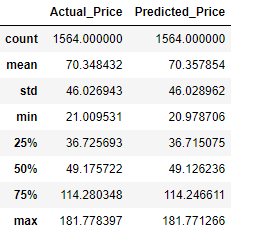
print("linear regression confidence: ", regression_confidence)linear regression confidence: 0.9998250952047488predicted=regression.predict(test_x) print(test_x.head())predicted.shape(1564,)dfr=pd.DataFrame({'Actual_Price':test_y, 'Predicted_Price':predicted}) dfr.head(10)dfr.describe()
print('Mean Absolute Error (MAE):', metrics.mean_absolute_error(test_y, predicted)) print('Mean Squared Error (MSE) :', metrics.mean_squared_error(test_y, predicted)) print('Root Mean Squared Error (RMSE):', np.sqrt(metrics.mean_squared_error(test_y, predicted)))dfr.describe()9. Final Outputplt.scatter(dfr.Actual_Price, dfr.Predicted_Price, color='Darkblue') plt.xlabel("Actual Price") plt.ylabel("Predicted Price") plt.show()
plt.plot(dfr.Actual_Price, color='red') plt.plot(dfr.Predicted_Price, color='lightblue') plt.title("$AAPL Prediction Chart") plt.legend();


Comments
Post a Comment