Short-term Stock Market Price Prediction using Deep Learning Models

This blog is about short-term stock market price trend prediction using a comprehensive deep learning LSTM model. Results show that the model achieves overall high accuracy for stock market trend prediction. The following end-to-end sequence provides the detailed Python/Jupyter workflow from data processing to prediction, including the data exploration:
1. Data Preparation Phase
#import libraries
import pandas as pd
import numpy as np
# To remove the scientific notation from numpy arrays
np.set_printoptions(suppress=True)
# install the nsepy library to get stock prices
!pip install nsepy
############################################
# Getting Stock data using nsepy library
from nsepy import get_history
from datetime import datetime
startDate=datetime(2021, 1,1)
endDate=datetime(2022, 10, 3)
# Fetching the data
StockData=get_history(symbol='INFY', start=startDate, end=endDate)
print(StockData.shape)
StockData.head()

# Creating a column as date
StockData['TradeDate']=StockData.index
# Plotting the stock prices
%matplotlib inline
StockData.plot(x='TradeDate', y='Close', kind='line', figsize=(20,6), rot=20)

2. Exploratory Data Analysis (EDA)
# Extracting the closing prices of each day
FullData=StockData[['Close']].values
print(FullData[0:5])
# Feature Scaling for fast training of neural networks
from sklearn.preprocessing import StandardScaler, MinMaxScaler
# Choosing between Standardization or normalization
#sc = StandardScaler()
sc=MinMaxScaler()
DataScaler = sc.fit(FullData)
X=DataScaler.transform(FullData)
#X=FullData
print('### After Normalization ###')
X[0:5]
Out[3]:
3. Fitting the RNN to the Training set
from keras.models import Sequential
from keras.layers import Dense
from keras.layers import LSTM
# Initialising the RNN
regressor = Sequential()
# Adding the First input hidden layer and the LSTM layer
# return_sequences = True, means the output of every time step to be shared with hidden next layer
regressor.add(LSTM(units = 10, activation = 'relu', input_shape = (TimeSteps, TotalFeatures), return_sequences=True))
# Adding the Second Second hidden layer and the LSTM layer
regressor.add(LSTM(units = 5, activation = 'relu', input_shape = (TimeSteps, TotalFeatures), return_sequences=True))
# Adding the Second Third hidden layer and the LSTM layer
regressor.add(LSTM(units = 5, activation = 'relu', return_sequences=False ))
# Adding the output layer
regressor.add(Dense(units = 1))
# Compiling the RNN
regressor.compile(optimizer = 'adam', loss = 'mean_squared_error')
##################################################
import time
# Measuring the time taken by the model to train
StartTime=time.time()
# Fitting the RNN to the Training set
regressor.fit(X_train, y_train, batch_size = 5, epochs = 100)
EndTime=time.time()
print("## Total Time Taken: ", round((EndTime-StartTime)/60), 'Minutes ##')
Epoch 1/100
61/61 [==============================] - 2s 5ms/step - loss: 0.2446
Epoch 2/100
61/61 [==============================] - 0s 5ms/step - loss: 0.0213
Epoch 3/100
61/61 [==============================] - 0s 5ms/step - loss: 0.0122
Epoch 4/100
61/61 [==============================] - 0s 5ms/step - loss: 0.0095
Epoch 5/100
61/61 [==============================] - 0s 5ms/step - loss: 0.0075
Epoch 6/100
61/61 [==============================] - 0s 5ms/step - loss: 0.0066
Epoch 7/100
61/61 [==============================] - 0s 5ms/step - loss: 0.0059
Epoch 8/100
61/61 [==============================] - 0s 5ms/step - loss: 0.0058
Epoch 9/100
61/61 [==============================] - 0s 5ms/step - loss: 0.0052
Epoch 10/100
61/61 [==============================] - 0s 5ms/step - loss: 0.0054
Epoch 11/100
61/61 [==============================] - 0s 5ms/step - loss: 0.0050
Epoch 12/100
61/61 [==============================] - 0s 5ms/step - loss: 0.0051
Epoch 13/100
61/61 [==============================] - 0s 5ms/step - loss: 0.0050
Epoch 14/100
61/61 [==============================] - 0s 5ms/step - loss: 0.0048
Epoch 15/100
61/61 [==============================] - 0s 5ms/step - loss: 0.0051
Epoch 16/100
61/61 [==============================] - 0s 5ms/step - loss: 0.0049
Epoch 17/100
61/61 [==============================] - 0s 5ms/step - loss: 0.0048
Epoch 18/100
61/61 [==============================] - 0s 5ms/step - loss: 0.0047
Epoch 19/100
61/61 [==============================] - 0s 5ms/step - loss: 0.0048
Epoch 20/100
61/61 [==============================] - 0s 5ms/step - loss: 0.0046
Epoch 21/100
61/61 [==============================] - 0s 5ms/step - loss: 0.0046
Epoch 22/100
61/61 [==============================] - 0s 5ms/step - loss: 0.0045
Epoch 23/100
61/61 [==============================] - 0s 5ms/step - loss: 0.0052
Epoch 24/100
61/61 [==============================] - 0s 5ms/step - loss: 0.0047
Epoch 25/100
61/61 [==============================] - 0s 5ms/step - loss: 0.0046
Epoch 26/100
61/61 [==============================] - 0s 5ms/step - loss: 0.0049
Epoch 27/100
61/61 [==============================] - 0s 5ms/step - loss: 0.0044
Epoch 28/100
61/61 [==============================] - 0s 5ms/step - loss: 0.0046
Epoch 29/100
61/61 [==============================] - 0s 5ms/step - loss: 0.0044
Epoch 30/100
61/61 [==============================] - 0s 5ms/step - loss: 0.0042
Epoch 31/100
61/61 [==============================] - 0s 5ms/step - loss: 0.0045
Epoch 32/100
61/61 [==============================] - 0s 5ms/step - loss: 0.0046
Epoch 33/100
61/61 [==============================] - 0s 5ms/step - loss: 0.0043
Epoch 34/100
61/61 [==============================] - 0s 5ms/step - loss: 0.0047
Epoch 35/100
61/61 [==============================] - 0s 5ms/step - loss: 0.0043
Epoch 36/100
61/61 [==============================] - 0s 5ms/step - loss: 0.0043
Epoch 37/100
61/61 [==============================] - 0s 4ms/step - loss: 0.0041
Epoch 38/100
61/61 [==============================] - 0s 5ms/step - loss: 0.0042
Epoch 39/100
61/61 [==============================] - 0s 5ms/step - loss: 0.0043
Epoch 40/100
61/61 [==============================] - 0s 5ms/step - loss: 0.0042
Epoch 41/100
61/61 [==============================] - 0s 5ms/step - loss: 0.0041
Epoch 42/100
61/61 [==============================] - 0s 5ms/step - loss: 0.0040
Epoch 43/100
61/61 [==============================] - 0s 5ms/step - loss: 0.0043
Epoch 44/100
61/61 [==============================] - 0s 5ms/step - loss: 0.0041
Epoch 45/100
61/61 [==============================] - 0s 5ms/step - loss: 0.0038
Epoch 46/100
61/61 [==============================] - 0s 5ms/step - loss: 0.0039
Epoch 47/100
61/61 [==============================] - 0s 5ms/step - loss: 0.0041
Epoch 48/100
61/61 [==============================] - 0s 5ms/step - loss: 0.0039
Epoch 49/100
61/61 [==============================] - 0s 5ms/step - loss: 0.0036
Epoch 50/100
61/61 [==============================] - 0s 5ms/step - loss: 0.0045
Epoch 51/100
61/61 [==============================] - 0s 5ms/step - loss: 0.0037
Epoch 52/100
61/61 [==============================] - 0s 5ms/step - loss: 0.0035
Epoch 53/100
61/61 [==============================] - 0s 4ms/step - loss: 0.0038
Epoch 54/100
61/61 [==============================] - 0s 4ms/step - loss: 0.0037
Epoch 55/100
61/61 [==============================] - 0s 5ms/step - loss: 0.0035
Epoch 56/100
61/61 [==============================] - 0s 4ms/step - loss: 0.0036
Epoch 57/100
61/61 [==============================] - 0s 5ms/step - loss: 0.0037
Epoch 58/100
61/61 [==============================] - 0s 5ms/step - loss: 0.0035
Epoch 59/100
61/61 [==============================] - 0s 5ms/step - loss: 0.0038
Epoch 60/100
61/61 [==============================] - 0s 5ms/step - loss: 0.0032
Epoch 61/100
61/61 [==============================] - 0s 5ms/step - loss: 0.0033
Epoch 62/100
61/61 [==============================] - 0s 5ms/step - loss: 0.0033
Epoch 63/100
61/61 [==============================] - 0s 5ms/step - loss: 0.0032
Epoch 64/100
61/61 [==============================] - 0s 5ms/step - loss: 0.0033
Epoch 65/100
61/61 [==============================] - 0s 5ms/step - loss: 0.0031
Epoch 66/100
61/61 [==============================] - 0s 5ms/step - loss: 0.0032
Epoch 67/100
61/61 [==============================] - 0s 5ms/step - loss: 0.0031
Epoch 68/100
61/61 [==============================] - 0s 5ms/step - loss: 0.0030
Epoch 69/100
61/61 [==============================] - 0s 5ms/step - loss: 0.0030
Epoch 70/100
61/61 [==============================] - 0s 5ms/step - loss: 0.0029
Epoch 71/100
61/61 [==============================] - 0s 5ms/step - loss: 0.0030
Epoch 72/100
61/61 [==============================] - 0s 5ms/step - loss: 0.0030
Epoch 73/100
61/61 [==============================] - 0s 5ms/step - loss: 0.0029
Epoch 74/100
61/61 [==============================] - 0s 5ms/step - loss: 0.0028
Epoch 75/100
61/61 [==============================] - 0s 5ms/step - loss: 0.0027
Epoch 76/100
61/61 [==============================] - 0s 5ms/step - loss: 0.0027
Epoch 77/100
61/61 [==============================] - 0s 5ms/step - loss: 0.0030
Epoch 78/100
61/61 [==============================] - 0s 5ms/step - loss: 0.0027
Epoch 79/100
61/61 [==============================] - 0s 5ms/step - loss: 0.0028
Epoch 80/100
61/61 [==============================] - 0s 5ms/step - loss: 0.0029
Epoch 81/100
61/61 [==============================] - 0s 5ms/step - loss: 0.0027
Epoch 82/100
61/61 [==============================] - 0s 5ms/step - loss: 0.0025
Epoch 83/100
61/61 [==============================] - 0s 5ms/step - loss: 0.0027
Epoch 84/100
61/61 [==============================] - 0s 5ms/step - loss: 0.0024
Epoch 85/100
61/61 [==============================] - 0s 5ms/step - loss: 0.0024
Epoch 86/100
61/61 [==============================] - 0s 4ms/step - loss: 0.0026
Epoch 87/100
61/61 [==============================] - 0s 5ms/step - loss: 0.0025
Epoch 88/100
61/61 [==============================] - 0s 5ms/step - loss: 0.0027
Epoch 89/100
61/61 [==============================] - 0s 5ms/step - loss: 0.0024
Epoch 90/100
61/61 [==============================] - 0s 5ms/step - loss: 0.0025
Epoch 91/100
61/61 [==============================] - 0s 5ms/step - loss: 0.0022
Epoch 92/100
61/61 [==============================] - 0s 5ms/step - loss: 0.0023
Epoch 93/100
61/61 [==============================] - 0s 5ms/step - loss: 0.0023
Epoch 94/100
61/61 [==============================] - 0s 4ms/step - loss: 0.0023
Epoch 95/100
61/61 [==============================] - 0s 5ms/step - loss: 0.0024
Epoch 96/100
61/61 [==============================] - 0s 5ms/step - loss: 0.0024
Epoch 97/100
61/61 [==============================] - 0s 5ms/step - loss: 0.0024
Epoch 98/100
61/61 [==============================] - 0s 5ms/step - loss: 0.0025
Epoch 99/100
61/61 [==============================] - 0s 5ms/step - loss: 0.0021
Epoch 100/100
61/61 [==============================] - 0s 5ms/step - loss: 0.0026
## Total Time Taken:  1 Minutes ##
4. Make Predictions & QC Analysis
predicted_Price = regressor.predict(X_test)
predicted_Price = DataScaler.inverse_transform(predicted_Price)
# Getting the original price values for testing data
orig=y_test
orig=DataScaler.inverse_transform(y_test)
# Accuracy of the predictions
print('Accuracy:', 100 - (100*(abs(orig-predicted_Price)/orig)).mean())
# Visualising the results
import matplotlib.pyplot as plt
plt.plot(predicted_Price, color = 'blue', label = 'Predicted Volume')
plt.plot(orig, color = 'lightblue', label = 'Original Volume')
plt.title('Stock Price Predictions')
plt.xlabel('Trading Date')
plt.xticks(range(TestingRecords), StockData.tail(TestingRecords)['TradeDate'])
plt.ylabel('Stock Price')
plt.legend()
fig=plt.gcf()
fig.set_figwidth(20)
fig.set_figheight(6)
plt.show()
Accuracy: 99.12386255608178

5. Output Data Visualization
TrainPredictions=DataScaler.inverse_transform(regressor.predict(X_train))
TestPredictions=DataScaler.inverse_transform(regressor.predict(X_test))
FullDataPredictions=np.append(TrainPredictions, TestPredictions)
FullDataOrig=FullData[TimeSteps:]
# plotting the full data
plt.plot(FullDataPredictions, color = 'blue', label = 'Predicted Price')
plt.plot(FullDataOrig , color = 'red', label = 'Original Price')
plt.title('Stock Price Predictions')
plt.xlabel('Trading Date')
plt.ylabel('Stock Price')
plt.legend()
fig=plt.gcf()
fig.set_figwidth(20)
fig.set_figheight(8)
plt.show()

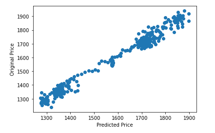
plt.scatter(FullDataPredictions,FullDataOrig)
plt.xlabel('Predicted Price')
plt.ylabel('Original Price')
Comments
Post a Comment